Anno 1800: Frame Analysis

Anno easily ranks among my favorite franchises. I still have fond memories of building beautiful medieval cities with dense waterways in 1404 and its Venice expansion. That was followed by Anno 2070, with its dual‑faction setup, world council, and an entirely new dimension with underwater biomes.

When the team at Ubisoft Mainz announced Anno 1800, I was thrilled. Pairing the Victorian era with the Anno formula felt like a perfect match. The game performed extremely well, reaching new markets and receiving four years of post‑launch content with new worlds and mechanics.

With Anno Pax 117: Romana right around the corner, it felt like a good time to dive into Anno 1800’s rendering. But we’re not here to talk business or analyze gameplay—you know the drill: we’re here to study the rendering.

Anno runs on a custom engine built specifically for the series. With tight constraints on mesh density, long view distances, dynamic buildings, terrain, and lighting, it’s a prime candidate for this kind of deep dive.

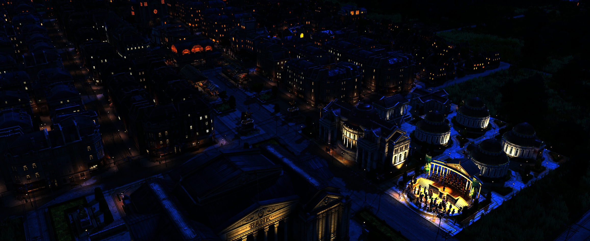
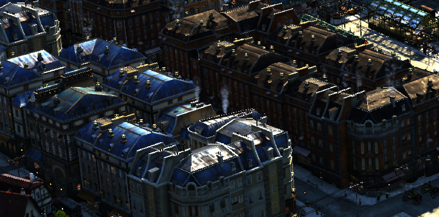
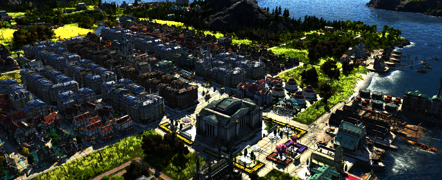
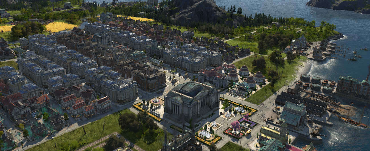
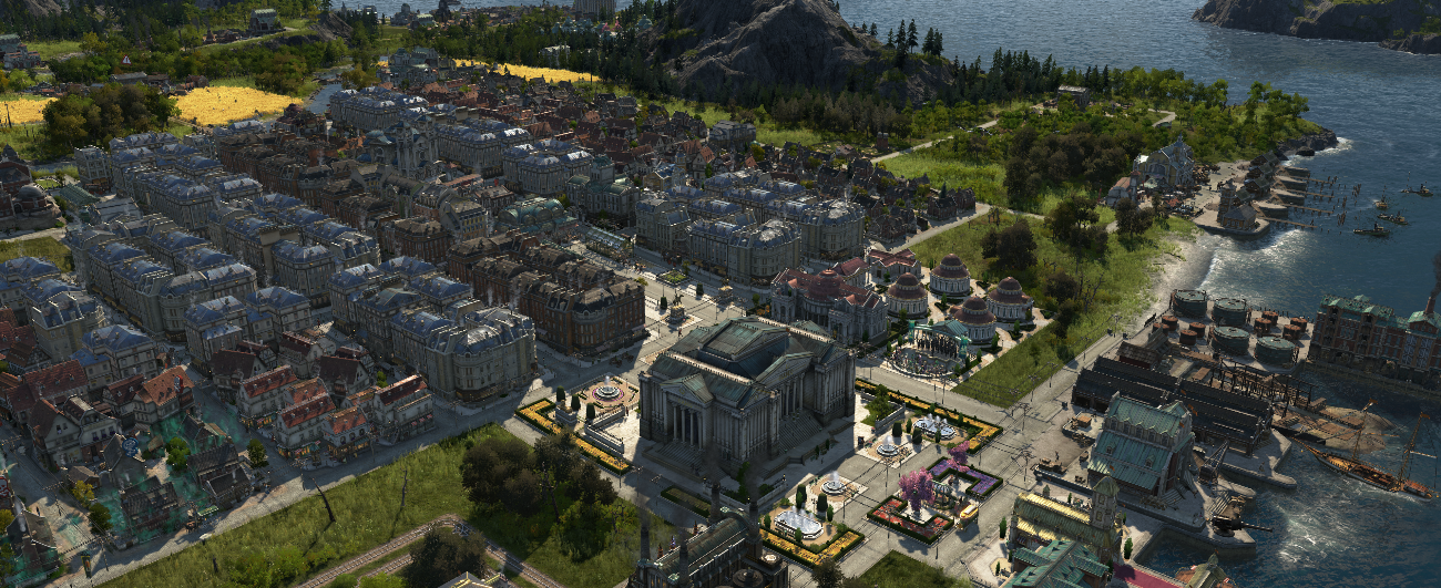
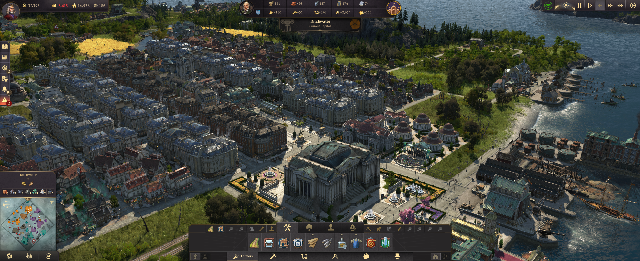
Here’s the scene we’ll analyze. I’ll also bring in two more examples later to highlight additional features.

Terrain Virtual Texture

Terrain in top‑down strategy games is tricky. You need huge coverage, high resolution, and enough variation to avoid repetition, which makes drawing the entire terrain every frame impractical. Caching helps, but brings its own problems like tile eviction and update rate. As the camera moves, tiles that scroll out of view must be dropped and new ones added. Picking what to evict (and when) takes careful tuning to keep the swap invisible. The hardest part, though, is reacting to edits like placing a road: those tiles must be refreshed promptly without stalling the frame.

One solution is to split up the terrain in a quadtree and maintain a pyramid of LOD tiles in the virtual texture. When tiles become dirty (from movement or edits), the renderer temporarily falls back to lower‑LOD tiles while higher‑LOD versions are updated in the background. Depending on platform and frame budget, only a handful of tiles may update per frame. This keeps the terrain looking coherent at all times, at the cost of brief blur during fast motion and large edits.

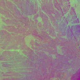
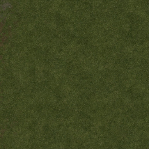
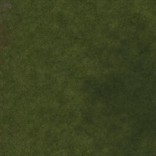
Looking at the frame, Anno 1800 seems to use a slightly different approach. When a terrain tile is rendered, it’s using a couple of textures. The first are large 8K textures covering the whole play area with all the islands: one for tint, and one for grit.

Looking at both together, we can see that the grit texture is mostly applied to coastal areas and seems to be a local enhancer. I’m unsure how this is used in practice, as despite the 8K resolution, the playfield is extremely large, making it comparatively low resolution when fully zoomed in. Hypothesis: it likely provides broad, low‑frequency variation and coastline breakup that complements the higher‑resolution node textures.

The second set of textures, referred to as “node textures,” echoes the virtual‑texture idea described above and provides the required high‑resolution detail for the terrain. I don’t believe Anno 1800 uses a quadtree, but it still renders and caches ahead of time the tiles’ textures. A buffer containing each tile’s node information is passed; it includes parameters to drive the rendering and, most importantly, an index into the virtual‑texture array.

To store the nodes’ textures, the engine uses an array of 763 slices of 512×512 textures (the slice count looks sized to fit the memory budget and update cadence).

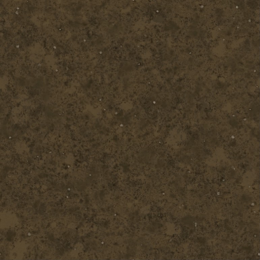
In that array we’ll find the diffuse and the specular. Note the compression, we’ll come back to that later.

We also have a normal and a tint map. Oddly, these are not provided through the array but via a regular binding. It’s not obvious why, as the infrastructure seems to be in place to support them in the array as well. Possibly a legacy binding choice or to allow different residency/update policies.

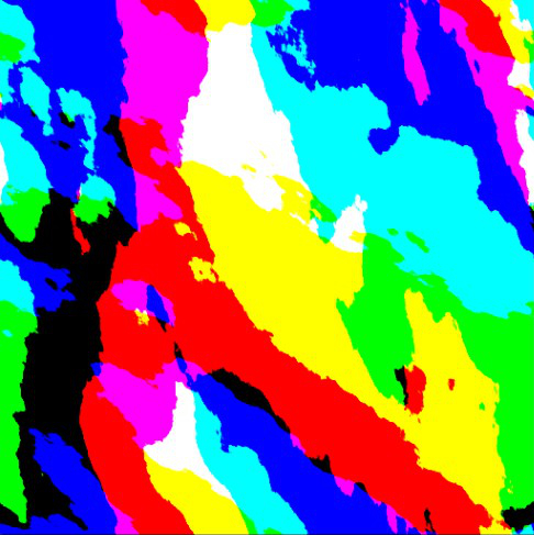
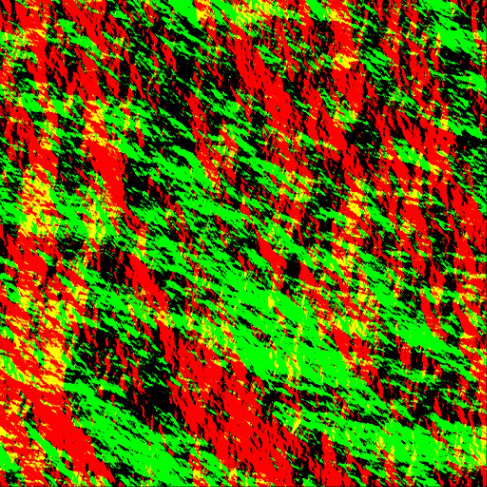
These detailed textures are updated at runtime and right at the start of the frame. Typically, the engine spreads the workload across multiple frames to lighten GPU pressure. This step—referred to as “baking”, appears to combine two stages: first render the ground layers from a material map, then apply decals on top.

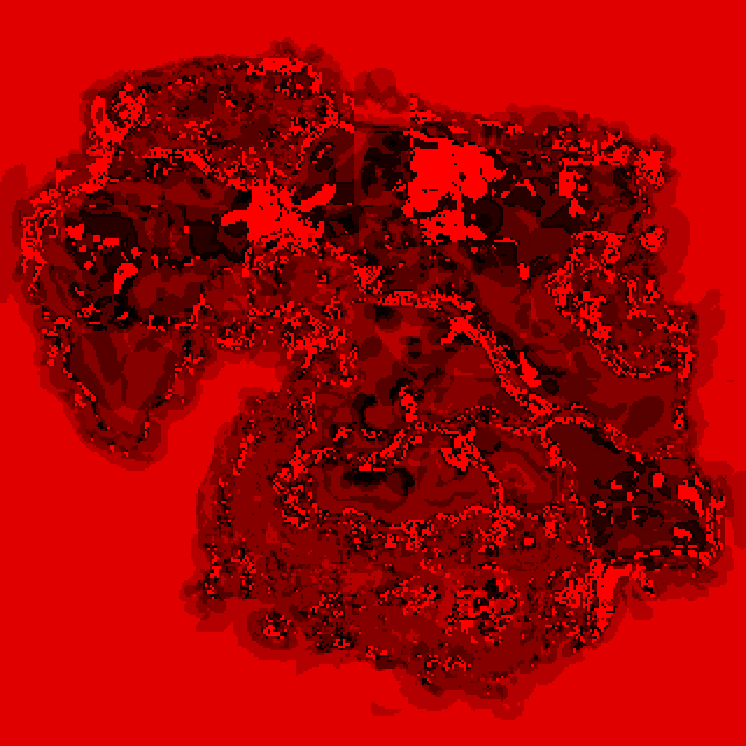
The map is stored as an R32_UINT, and is likely used as a bitfield to pick which layers to blend. From observation, around ten layers typically contribute to a tile. Many layers contribute only marginally or end up occluded, which suggests they act as localized transitions or provide headroom for edits (roads, terrain painting) without rebaking the full set.

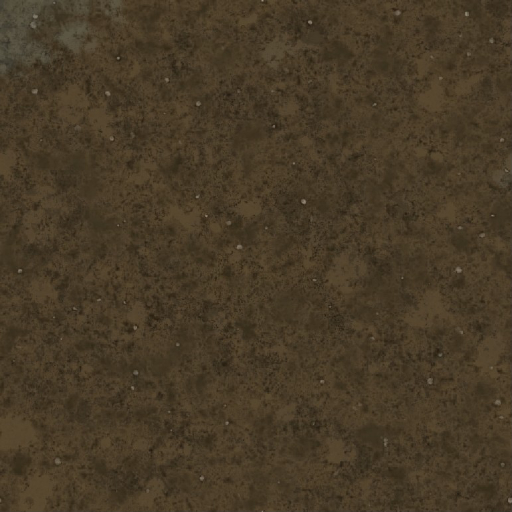
Here is an example: this tile is built using eleven layers. I’ll show only the steps that change the result.

The final step in the process is to generate mipmaps for the textures and compress the diffuse texture using a custom compute shader. Based on the shader’s structure and the visual result, it’s most likely using BC7 compression.

Sky cubemap

Right after updating the virtual texture, the engine renders a dynamic sky cubemap used for diffuse irradiance (and potentially reflections).

The cubemap is generated by a shader that models atmospheric scattering and includes a sun disk.

I reimplemented the shader in Shadertoy if you want to see it live.

The sky is rendered at 64×64 and then passed to a mip generator to produce 32×32 and 16×16 levels. Because diffuse irradiance is low frequency, this resolution is enough and inexpensive.

Mip generation

The mip generator itself isn’t unusual, but it’s a good candidate for a compact shader IR walkthrough: it’s small, self‑contained, and shows that shader assembly isn’t that scary.

//
// Generated by Microsoft (R) HLSL Shader Compiler 10.1
//
//
// Note: shader requires additional functionality:
//       Typed UAV Load Additional Formats
//
//
// Buffer Definitions:
//
// cbuffer cbMipGenerator
// {
//
//   float2 cMipGenDstTexelSize;        // Offset:    0 Size:     8
//   float2 cMipGenSrcSize;             // Offset:    8 Size:     8
//
// }
//
//
// Resource Bindings:
//
// Name                                 Type  Format         Dim      ID      HLSL Bind  Count
// ------------------------------ ---------- ------- ----------- ------- -------------- ------
// ]                     UAV  float4          2d      U0             u0      1
// cMipGenTextureSrc                     UAV  float4          2d      U1             u1      1
// cbMipGenerator                    cbuffer      NA          NA     CB0            cb0      1
//
//
//
// Input signature:
//
// Name                 Index   Mask Register SysValue  Format   Used
// -------------------- ----- ------ -------- -------- ------- ------
// no Input
//
// Output signature:
//
// Name                 Index   Mask Register SysValue  Format   Used
// -------------------- ----- ------ -------- -------- ------- ------
// no Output
      0x00000000: cs_5_1
      0x00000008: dcl_globalFlags refactoringAllowed | allResourcesBound
      0x0000000C: dcl_constantbuffer CB0[0:0][1], immediateIndexed, space=0
      0x00000028: dcl_uav_typed_texture2d (float,float,float,float) U0[0:0], space=0
      0x00000044: dcl_uav_typed_texture2d (float,float,float,float) U1[1:1], space=0
      0x00000060: dcl_input vThreadID.xy
      0x00000068: dcl_temps 6
      0x00000070: dcl_thread_group 8, 8, 1
   0  0x00000080: utof r0.xy, vThreadID.yxyy
   1  0x00000090: mul r0.zw, CB0[0][0].yyyx, l(0.000000, 0.000000, 0.250000, 0.250000)
   2  0x000000C0: mad_sat r0.xy, r0.xyxx, CB0[0][0].yxyy, r0.zwzz
   3  0x000000EC: mul r0.zw, r0.xxxy, CB0[0][0].wwwz
   4  0x00000110: ftoi r1.xyzw, r0.wzzz
   5  0x00000124: round_ni r0.zw, r0.zzzw
   6  0x00000138: mad r0.xy, r0.xyxx, CB0[0][0].wzww, -r0.zwzz
   7  0x00000168: ld_uav_typed r2.xyzw, r1.xwww, U1[1].xyzw
   8  0x00000188: iadd r3.xyzw, r1.xwxw, l(0, 1, 1, 0)
   9  0x000001B0: ld_uav_typed r4.xyzw, r3.xyyy, U1[1].xyzw
  10  0x000001D0: ld_uav_typed r3.xyzw, r3.zwww, U1[1].xyzw
  11  0x000001F0: iadd r1.xyzw, r1.xyzw, l(1, 1, 1, 1)
  12  0x00000218: ld_uav_typed r1.xyzw, r1.xyzw, U1[1].xyzw
  13  0x00000238: add r0.zw, -r0.yyyx, l(0.000000, 0.000000, 1.000000, 1.000000)
  14  0x00000264: mul r5.x, r0.w, r0.z
  15  0x00000280: mul r0.zw, r0.xxxy, r0.zzzw
  16  0x0000029C: mul r4.xyzw, r4.xyzw, r0.zzzz
  17  0x000002B8: mad r2.xyzw, r5.xxxx, r2.xyzw, r4.xyzw
  18  0x000002DC: mad r2.xyzw, r0.wwww, r3.xyzw, r2.xyzw
  19  0x00000300: mul r0.x, r0.x, r0.y
  20  0x0000031C: mad r0.xyzw, r0.xxxx, r1.xyzw, r2.xyzw
  21  0x00000340: store_uav_typed U0[0].xyzw, vThreadID.xyyy, r0.xyzw
  22  0x0000035C: ret
// Approximately 23 instruction slots used

In this form, the shader is composed of two parts:

• Metadata that describes resource bindings
• The compiled shader instructions

The compiled form here is an intermediate representation that drivers then use to generate hardware‑specific code.

The listing is DXBC, used in DirectX 9–11. DirectX 12 uses DXIL, which offers more compiler flexibility but is harder to read. If you want to learn more about it I recommend checking this article: https://devlog.hexops.com/2024/building-the-directx-shader-compiler-better-than-microsoft/

Checking the metadata, we learn that our shader is reading from:

• A source texture named cMipGenTextureSrc bound to u1
• A destination texture named cMipGenTextureSrc bound tou0
• A constant buffer containing bound to cb0 information about:
  • The destination texture texel size cMipGenDstTexelSize
  • The source texture size cMipGenSrcSize

At the top of our shader, we have some information about its geometry (8, 8, 1) and its version (cs_5_1), as well as the definition of our inputs. We also learn from dcl_temps that our shader is going to use 6 temporary registers (r0-r5)

      0x00000000: cs_5_1
      0x00000008: dcl_globalFlags refactoringAllowed | allResourcesBound
      0x0000000C: dcl_constantbuffer CB0[0:0][1], immediateIndexed, space=0
      0x00000028: dcl_uav_typed_texture2d (float,float,float,float) U0[0:0], space=0
      0x00000044: dcl_uav_typed_texture2d (float,float,float,float) U1[1:1], space=0
      0x00000060: dcl_input vThreadID.xy
      0x00000068: dcl_temps 6
      0x00000070: dcl_thread_group 8, 8, 1

Next up is the generation of the sampling UV. The goal is to transform the ThreadID which represent the absolute coordinate of a pixel in the destination texture into a normalized value we can then remap to the source texture. We can note in the instruction 1 the multiplication by 0.25 of the destination texel size that will be used just after to offset the sample to the center of the texel.

   0  0x00000080: utof r0.xy, vThreadID.yxyy
   1  0x00000090: mul r0.zw, CB0[0][0].yyyx, l(0.000000, 0.000000, 0.250000, 0.250000)
   2  0x000000C0: mad_sat r0.xy, r0.xyxx, CB0[0][0].yxyy, r0.zwzz

The UV value is then remaped to the source texture coordinate and converted to a integer for use in sampling

3  0x000000EC: mul r0.zw, r0.xxxy, CB0[0][0].wwwz
4  0x00000110: ftoi r1.xyzw, r0.wzzz

That pixel coordinate in the source texture that we just calculated can now be used to sample the source pixel value.

We take 4 samples of the source texture:

• r2 being the upper left corner
• r4 being the upper right (note the addition in 8 shifting the coordinates)
• r3 being the bottom left
• r1 being the bottom right (once again we shift the coordinates in 11)

   7  0x00000168: ld_uav_typed r2.xyzw, r1.xwww, U1[1].xyzw
   8  0x00000188: iadd r3.xyzw, r1.xwxw, l(0, 1, 1, 0)
   9  0x000001B0: ld_uav_typed r4.xyzw, r3.xyyy, U1[1].xyzw
  10  0x000001D0: ld_uav_typed r3.xyzw, r3.zwww, U1[1].xyzw
  11  0x000001F0: iadd r1.xyzw, r1.xyzw, l(1, 1, 1, 1)
  12  0x00000218: ld_uav_typed r1.xyzw, r1.xyzw, U1[1].xyzw

In case you didn’t catch it before, the shader is performing a bilinear interpolation, meaning the next step is to calculate the weights for each sample before we bring them together. This is done using the fractional part of the pixel coordinate.

   5  0x00000124: round_ni r0.zw, r0.zzzw
   6  0x00000138: mad r0.xy, r0.xyxx, CB0[0][0].wzww, -r0.zwzz
  13  0x00000238: add r0.zw, -r0.yyyx, l(0.000000, 0.000000, 1.000000, 1.000000)

The samples can then be added together using the weights calculated above.

  14  0x00000264: mul r5.x, r0.w, r0.z
  15  0x00000280: mul r0.zw, r0.xxxy, r0.zzzw
  16  0x0000029C: mul r4.xyzw, r4.xyzw, r0.zzzz
  17  0x000002B8: mad r2.xyzw, r5.xxxx, r2.xyzw, r4.xyzw
  18  0x000002DC: mad r2.xyzw, r0.wwww, r3.xyzw, r2.xyzw
  19  0x00000300: mul r0.x, r0.x, r0.y
  20  0x0000031C: mad r0.xyzw, r0.xxxx, r1.xyzw, r2.xyzw

Finally, we write the resulting value to our destination texture, and return

  21  0x00000340: store_uav_typed U0[0].xyzw, vThreadID.xyyy, r0.xyzw
  22  0x0000035C: ret

Depth Prepass

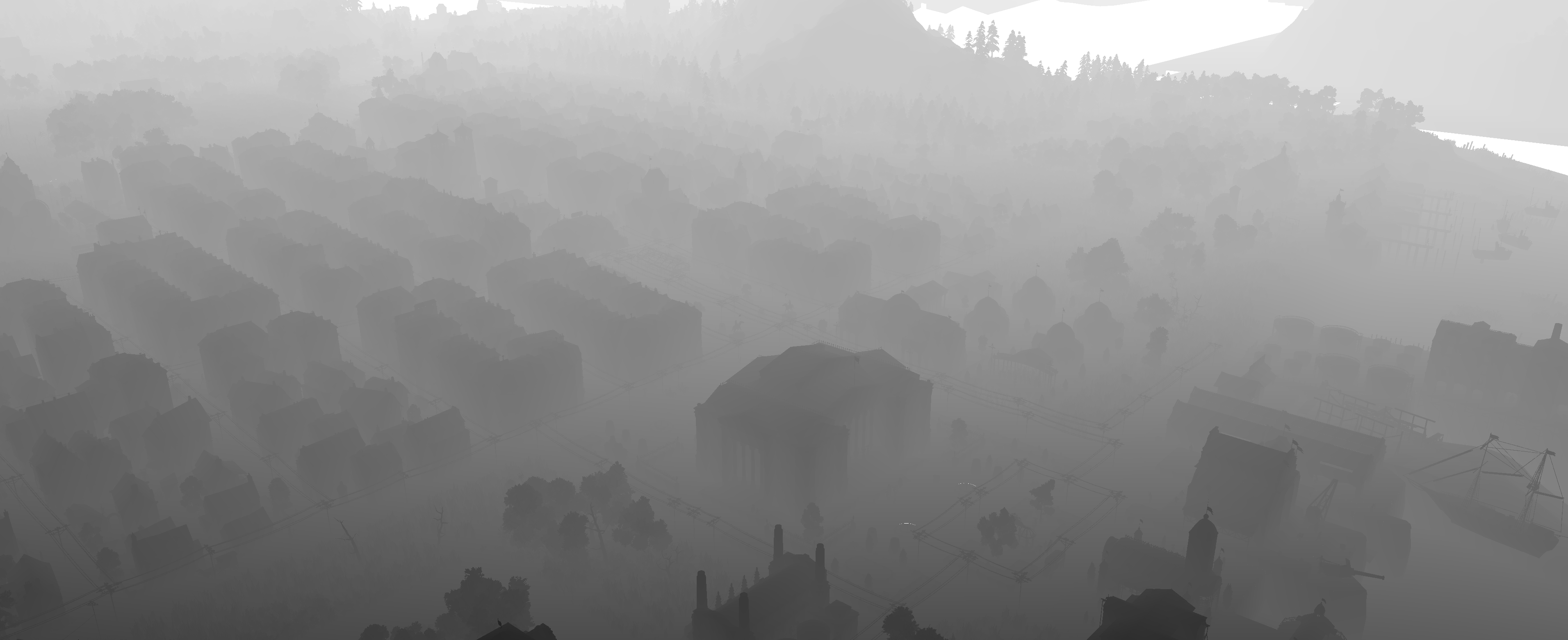
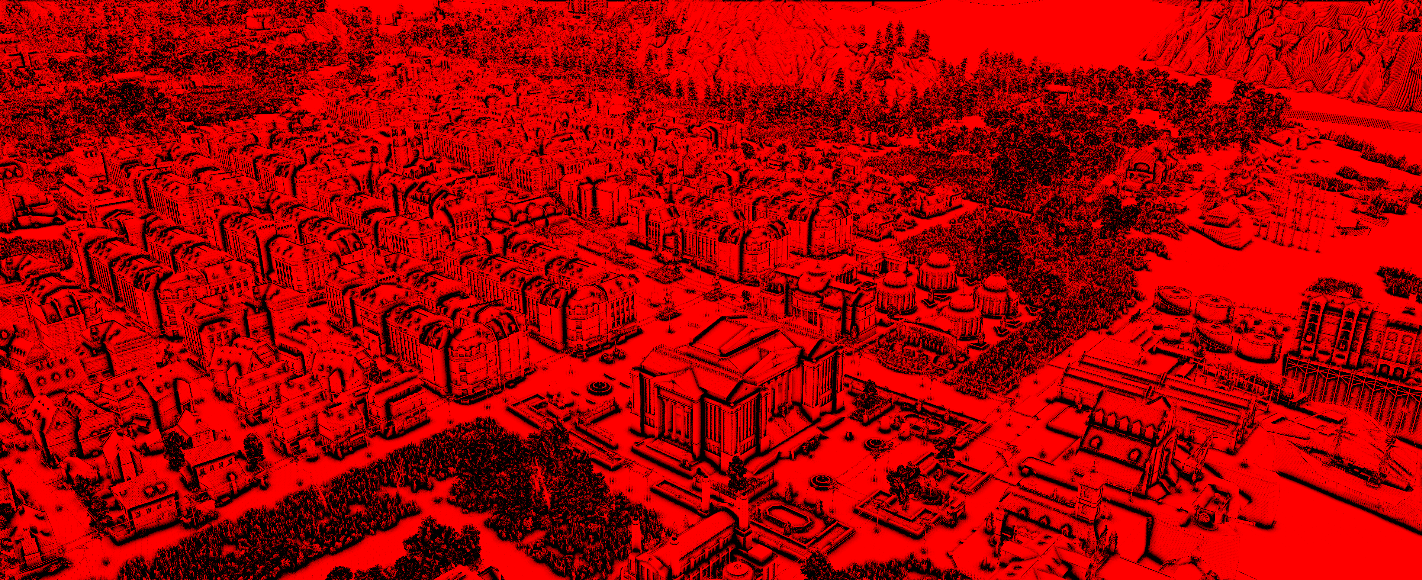
With all the preparation work out of the way, we can start the rendering of the main image. Anno 1800 uses a forward rendering pipeline starting with a predepth pass. During this pass, three targets are being written to.

With the preparation work done, we can start rendering the main image. Anno 1800 uses a forward rendering pipeline, starting with a depth prepass. In this pass, three targets are being written to, which helps reduce overdraw (early‑Z/Hi‑Z) and stage surface data for later passes in a scene that’s both dense and layered.

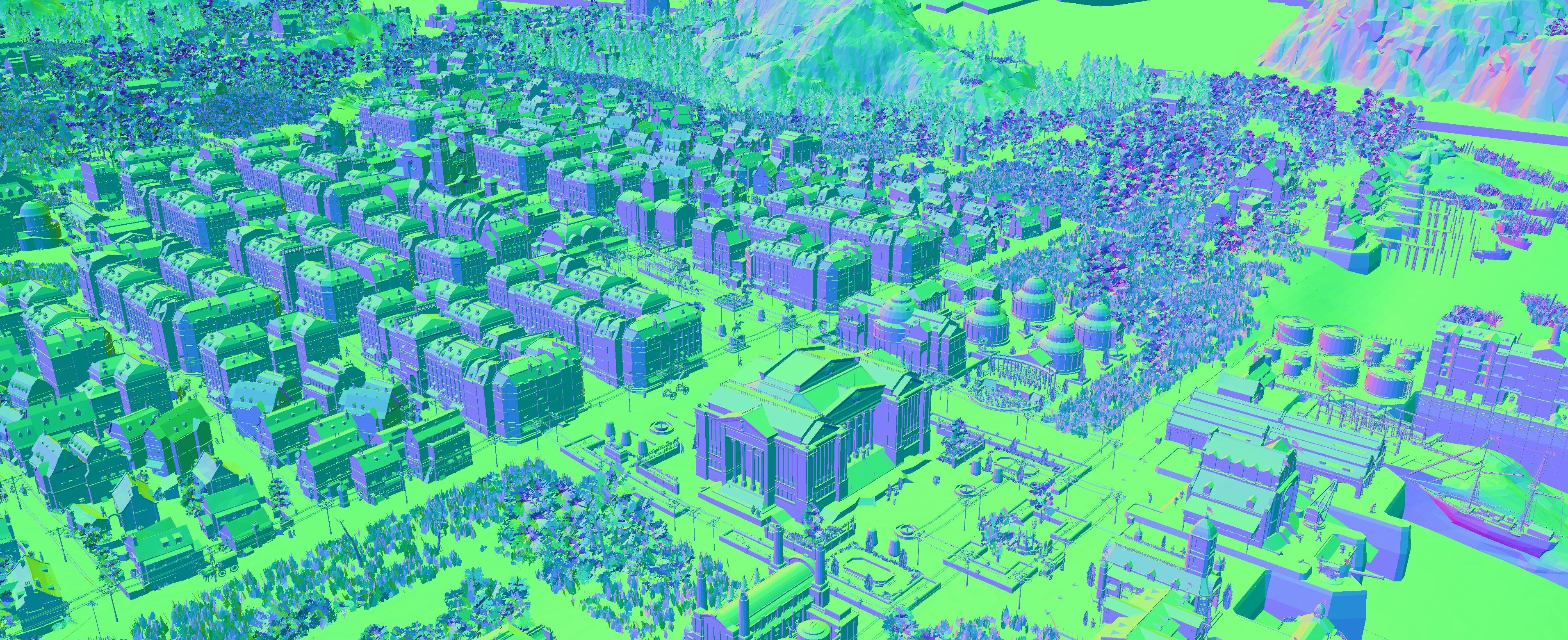
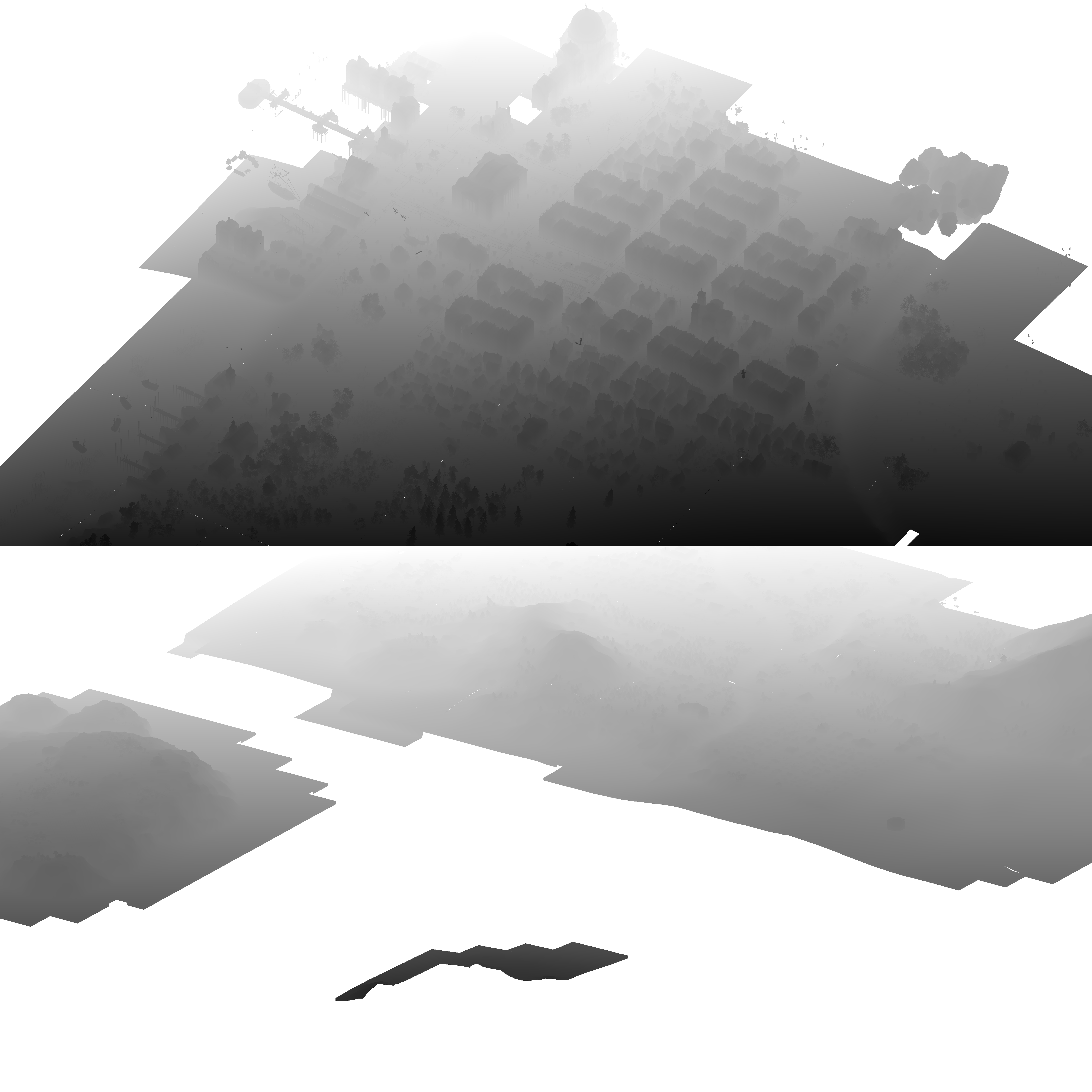
One, as expected is depth.

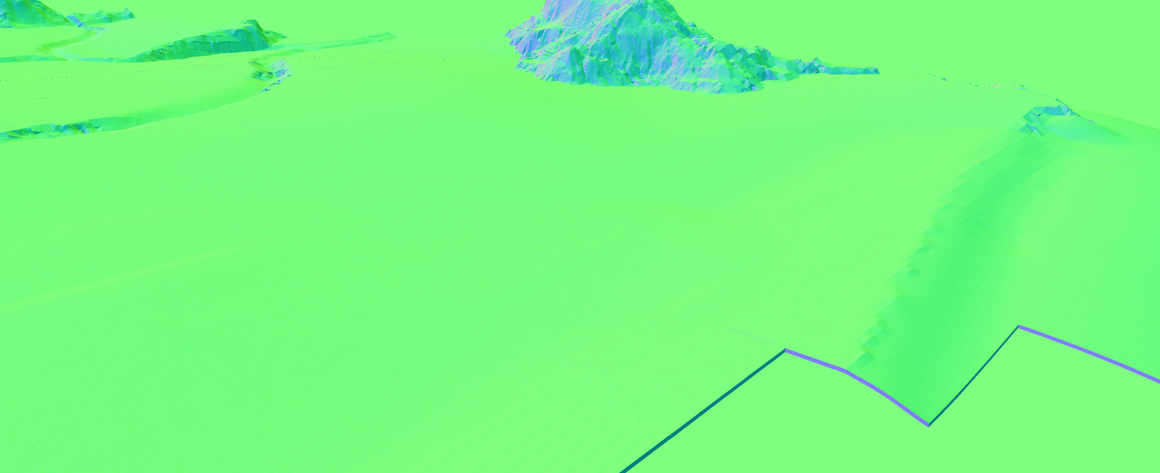
Another one is the normals.

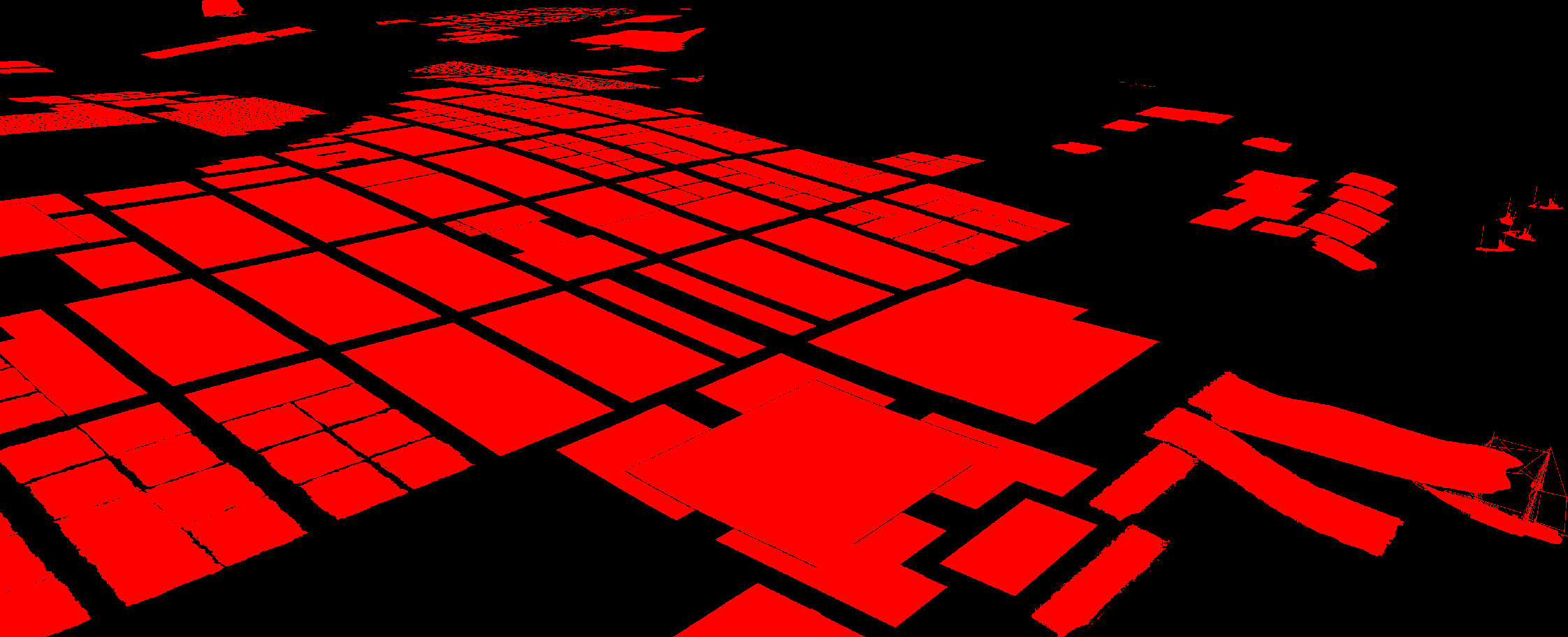
Finally, stencil. It tags classes of objects for selective processing later (e.g., water interactions, object‑specific effects).

Here are some I could identify:

• Default - 0x00
• Building pad - 0x10
• Building water (fountains, pond) - 0x11
• Boat - 0x01

Shadows

Anno is using two shadow cameras rendered to the same large target packed vertically in a single shadow map atlas.

Note how the two cameras have very different inclinations. Likely a compromise between close‑range fidelity and broad terrain readability. The top one provides higher quality with a tighter frustum for close‑ups, while the bottom one is used for more dramatic, wide‑area terrain shadows when you’re further away.

Another point of interest in the shadow rendering is its heavy use of indirect drawing.

It starts by drawing the terrain and a few miscellaneous meshes, then performs compute‑driven frustum culling of the rest (buildings, boats, etc.) to populate the indirect argument buffer and the per‑instance data.

This GPU‑driven approach can be very effective, but here it appears constrained by non‑bindless resource binding: an ExecuteIndirect is issued per mesh instance, each carrying its own bindings, which leads to many small draws. This could benefit from bindless/descriptor indexing for resources, enabling one (or a few) ExecuteIndirect calls that the GPU expands into many draws.

Still, this is miles better than CPU‑side culling and draw generation, and it’s always good to see indirect used effectively.

Color pass

It’s finally time to render color. Nothing exotic here: the scene is rendered to a multisampled R16G16B16A16_FLOAT HDR target (4× MSAA in this capture), which suits Anno’s dense geometry and alpha‑tested edges.

Towards the end of the main color pass, water and other transparent elements are rendered. They were not part of the depth prepass; depth writes happen here to keep correct ordering for transparency.

The stencil is also updated to account for additional classifications:

• 3D icons - 0x88
• Sea - 0x04

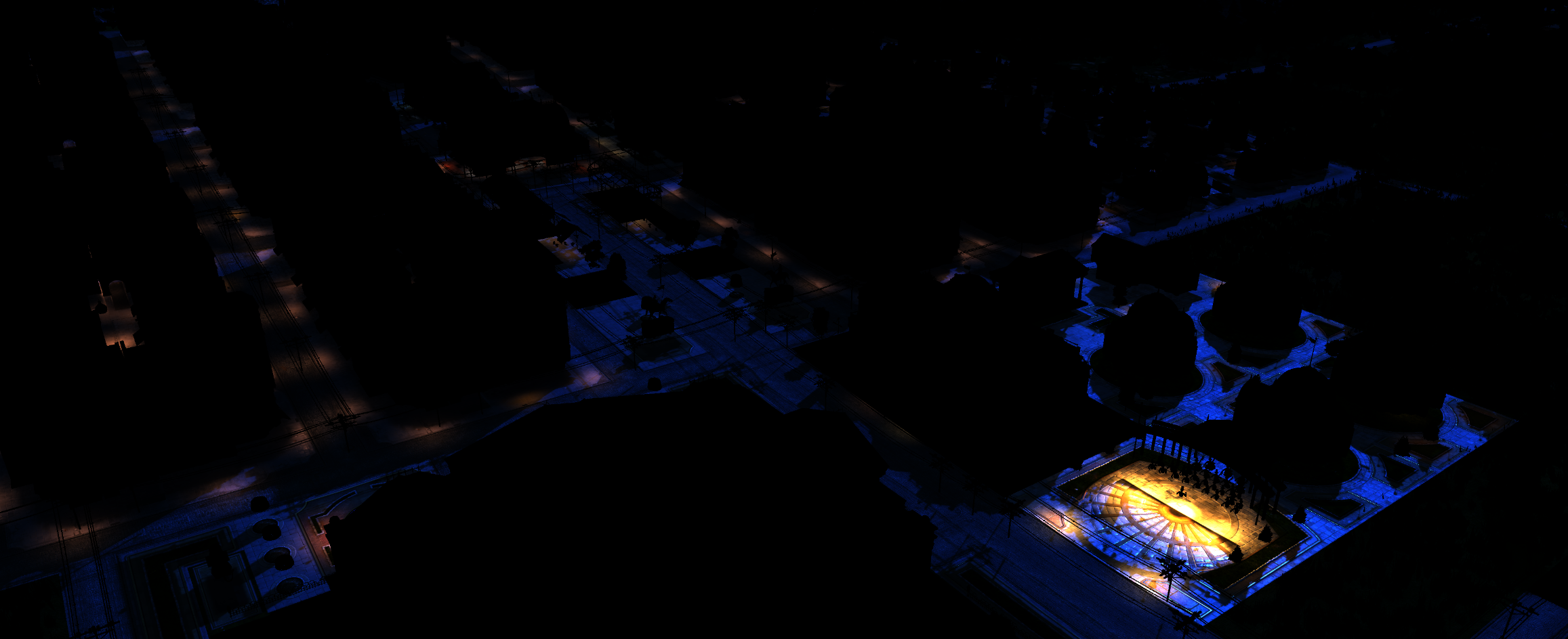
Let’s switch to night mode to quickly look at lighting. It looks like a forward+‑style approach, as each draw references four light‑related buffers:

• LightClusterBuffer: Most likely encode which light falls into which cluster
• LightIndexTex : Some kind of indirection texture
• PointLights: 2 float4 per light, with a maximum of 2048 sources
• SpotLights: 3 float4 per light, with a maximum of 1365 sources (the buffer can contain 4096 float4 elements, but that’s obviously non divisible by 3)

As for windows, an emissive mask texture is passed to the shader.

@# Particles

We find another neat trick in particle rendering: the system pushes most animation work to the GPU using precomputed curves and per‑instance data.

Let’s take a closer look at one chimney smoke stack to understand what’s going on. This particle system starts as a simple quad with a 16‑bit index buffer and a float2 vertex buffer containing only positions.

The draw draw call uses DrawIndexedInstanced. An instance represents a particle; in this case we have 52. Similar systems aren’t merged: one system equals one draw call.

The magic happens in the vertex shader, where a set of precomputed textures and constants transform and animate each quad.

These notes reflect best‑effort reverse engineering (resources + disassembly). The shader is ~350 instructions; details may vary, but the overall model should be accurate.

First, a root constant is provided to the shader. This root constant contains 3 values.

• The index of that particle system type
• The index of that particle system
• The index of that particle system draw call

Using the particle system type index, we can find some information about our particle system in the ParticlePerConfigDatabuffer. This buffer contains information about every particle system type in our frame, with a maximum of 128 types. We’ll find:

• Information about our movie animation such as a speed factor or number of frames. A movie refers to the animated texture played on the quad.
• Number of particles emitted by the system.
• Number of frames in the system, think of it as the lifetime of a particle
• Bounding box and emitter position in that bounding box.

We can also get some information about the specific particle system using its respective index in the ParticlePerConfig buffer.

• Transformation matrix
• Color modifier
• Scale
• Age

ParticlePerDrawCall appears to hold flags only. The last two buffers support up to 512 systems and both seem to be CPU‑updated every frame

Next let’s check the textures, the first one, ParticleBornTex contains information about:

• X: The particle lifetime offset
• Y: Some systems uses it, seems to be an offset of some kind
• Z: Particle lifetime. As far as I could tell, this value is never used and the particle always use the value from the config data buffer

Then we have a set of 4 textures that contains the:

• Color over time ParticleColorTex
• Position over time ParticlePositionTex
• Rotation over time ParticleRotationTex
• Scale over time ParticleScaleTex

These textures are laid out as one line per particle and one column per frame/time sample. The different bar lengths/offsets align with the animation length and lifetime from the born/config data.

If at a given frame a particle falls between its death and next emission window, the shader effectively samples undefined data and places the quad off‑screen. Using the lifetime here to collapse the quad might avoid that, but the practical gain is likely negligible.

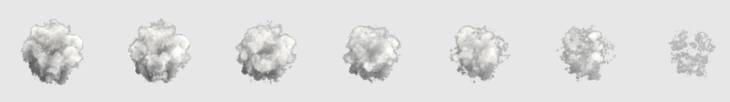
Finally, in the pixel shader, the flipbook texture (ParticleMovieTex) provides the visual; optional normal and motion textures can be sampled as well.

Overall, the system is nicely tuned to its constraints—handling a large on‑screen count (roughly 400 in this capture) by keeping geometry minimal, instancing per particle, and driving animation from compact, precomputed textures.

Post Processing

The post‑processing stack in Anno 1800 is quite light and is achieved in only seven draw calls.

It starts with a bloom pass, extracting high‑luminance areas from the multisampled scene. It is followed by a separable blur filter, starting with the horizontal pass. And then another pass of the same separable blur filter.

Next, the multisampled texture is resolved, converted back to LDR via tone mapping, and the blurred bloom is composited on top.

For the final step of the post-processing a color grading LUT is applied.

User Interface

The last step in the pipeline is rendering the user interface a critical step in Anno.

The interface is built with a tool/library called Phoenix, a shared Ubisoft technology (used by other games like Rainbow Six Siege). You can learn more about it and some of its design decisions here.

Rendering‑wise, Phoenix renders the UI with many DrawIndexedInstanced calls—about 500. In this capture, instancing isn’t used (instance count is 1), so each draw renders a single UI element.

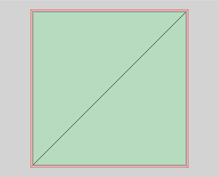
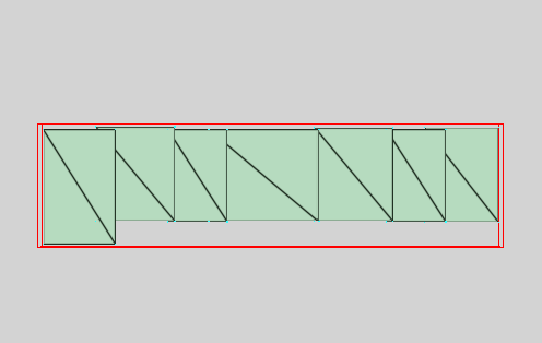
I want to highlight a technique commonly used in UI rendering to get perfect‑looking boxes, buttons, and other rectangular elements: nine‑slicing.

This technique is used whenever you need an element that can be resized while retaining its styling. If you non‑uniformly scale an element with rounded corners, the corners go out of proportion: nine‑slicing avoids that.

By splitting your element into nine slices, you render each independently: corners copy the texture as‑is; borders stretch along one axis; the center stretches along both axes. I say “stretch,” but you can also repeat the texture, for example to preserve a pattern.

This technique is extremely powerful, and we can see it in action here, implemented directly in the mesh used for rendering.

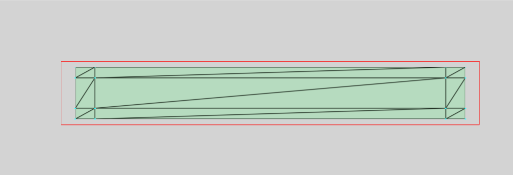
As you can see, the mesh is split into nine sections (corners, borders, and center), with UVs set to reflect the mapping in the texture.

I also want to quickly focus on text rendering.

The text is rendered using a quad per glyph. These quads are generated on the CPU and pushed as‑is to the GPU for rendering, the GPU being only responsible for screen space transformation. A glyph is rendered using a distance field sampled from a master font atlas. That atlas contains a lot of empty space(!) the Latin letters in lowercase and uppercase, some accents, some Cyrillic letters, numbers, and symbols.

Although a distance‑field texture is used here (as opposed to a texture per font size), making it much more efficient to scale glyphs up and down, the developers chose a single‑channel distance field. By contrast, multi‑channel distance fields (MSDF) preserve sharp corners better.

You can learn more about this using these resources:

• The original article by Valve on using distance fields
• Chlumský’s master thesis on using multi-channel distance fields
• A tool to generate these multi-channel distance fields

Wave simulation

The frame is technically complete, but while we were looking at the shadow pass, work continued in parallel. Anno 1800 uses the GPU’s async‑compute capabilities to offload compute‑intensive tasks and overlap them with graphics work.

The first is the wave simulation. As with many games, it uses an FFT‑based ocean approach.

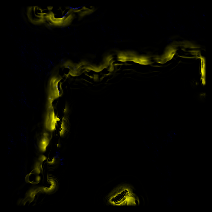
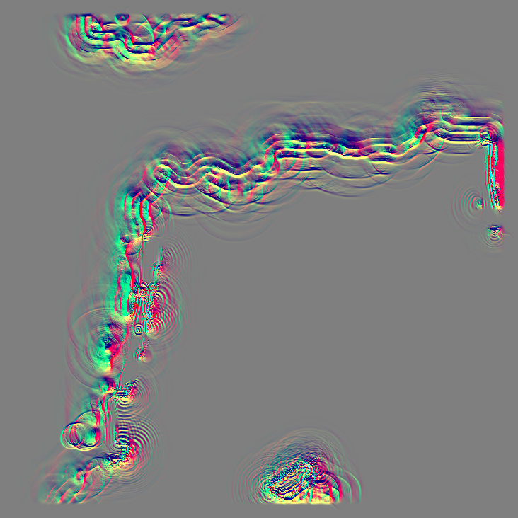
In this capture it first generates the large‑wave displacement map and its mipmaps, as well as the large‑wave surface‑gradient map and its mipmaps.

Following the same approach, the small‑wave displacement and gradient maps are generated too. Despite being the same size (512×512), the small‑wave displacement maps are compressed in BC6 and split into XZ and Y components, likely for efficient packing and precision.

The results are then used to calculate what is likely a local simulation around the islands/shorelines. This is rendered into two 2048×2048 textures containing a displacement plus a divergence/foam/pressure‑like term, and a separate motion (velocity) map, which is sampled during water shading for detail.

SSAO

The other task running on async compute is SSAO.

It’s a classic implementation: SSAO is computed at quarter resolution relative to the screen, using depth (and likely normals) from the prepass to control cost and noise. The result is then upsampled to full resolution, where a two‑pass separable blur (likely edge‑aware) is applied to reduce noise while preserving edges.

Conclusion

Anno 1800’s frame is a good reminder that mature pipelines don’t need to be flashy to be effective: they need to be coherent. Across the frame, you see pragmatic choices that fit the game’s constraints (huge scenes, dense assets, readability) and still leave room for flourishes.

It’s still refreshing from time to time to come back to a game running its own engine and pipeline. An engine tailormade for a specific game, built over generations of titles, that fits perfectly its constraints and serves the game’s needs.